Path analysis of Stock trends

If you’re reading the series on development of the stock trend screener for the first time, please go through the following articles first to develop some context:
1. AC and LR strategy for stock trend detection, backtested (naively): https://alphaleaks.info/stock-trend-backtest-using-ac-and-lr-criteria/
2. Improvement of the previous backtest: https://alphaleaks.info/stock-trend-backtest-using-ac-and-lr-criteria/

INTRODUCTION

This is the penultimate article exploring stock trend detection strategies. The first article of this series describing the rationale behind the AC and LR based strategy can be found HERE. And the next article discussing and addressing the limitations of the naïve backtest can be found HERE.
Since we have found promising results with some of the strategies, in this article we take our efforts a bit further, analyzing the potential paths our strategy can take over the years, if we stuck to these criteria.

RATIONALE

The crux of path analysis is introducing randomness into the original effect that we find in the original backtest. Usually, backtests lead to a single historical equity curve, which may be taken as the whole and absolute truth for future forecasts (the idiotic way 9:20 came into play). Or the backtest equity curve may be imagined as a series of individual returns which may come and go at random.
Having this foresight, you can imagine that if due to random chance, a series of negative returns clustered together (maybe due to change in market behavior), the cumulative drawdown in the equity curve might be enough to wipe you out. Thus, you realize the importance of path testing where the frequency distribution of the returns varies very little, but the order in which they occur can be varied randomly. This can potentially lead to massive changes in the shape of the cumulative equity curve.
By conducting path analysis of thousands of equity curves (based on the returns distribution of your original curve), you can derive an idea of the probability of you flying high or you being buried deep underground.

These paths can be derived via two methods:
1. Monte Carlo: In this you graph out the histogram of your return stream-> observe the characteristics of the shape of the histogram-> come up with parameters that best describe the histogram shape (central tendency, dispersion, skew, kurtosis etc., read more about these HERE)-> Use these parameters to derive random values which fit the frequency distribution of your original return stream-> Compute paths by cumsumming these random returns-> Graph these out and observe how many times you could have gone under.

2. Bootstrapping: In this, you resample with replacement, your original return stream many times, and then cumsum and graph them out. The benefit of this method is that it is simple and intuitive, and you don’t make any assumptions about the underlying frequency distribution. I use this method to conduct path analysis of our stock trend strategies.

METHODOLOGY

If you paid attention to the methodology of the previous article, you would realize that since we are randomly selecting one stock from the list of stocks fulfilling buy criteria on any one day, we already are generating a random data stream. On top of this randomness, we are adding another layer, by conducting the boot strapping.
Each market capitalization universe was subjected to each of the 4 signals described in the previous article, and returns were calculated for 5, 20 and 60 day holding periods respectively.

1. Thus we have 4 (market caps)*4(signals)*3(holding periods)=48 separate return curves.

2. Each of these streams were instructed to randomly select a stock from the list of stocks fulfilling buy criteria, and holding them for the respective holding period. This random selection was conducted 500 times for all 48 return curves.

3. Each of the these randomly selected return curves was further resampled 10 times (bootstrapping) [tried 100 times, but RAM choked], to finally generate 5000 separate return streams for each of the 48 original strats.

4. Since we are looking to reduce risk and not maximize returns with this exercise, curves with final returns in the 90th-100th percentiles were removed to improve the reliability of summary statistics.

5. A variety of statistical testing can be done on these, but for sake of simplicity, today we will just graph them out and obtain summary statistics of the final returns and drawdowns of each of these streams.

RESULTS

Before we look at the graphs, let’s have a look at the statistics for final returns and drawdowns.
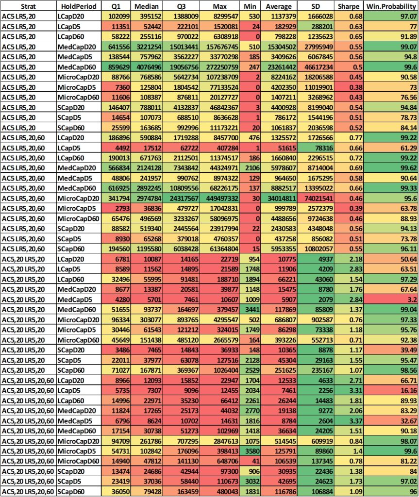
1. Final Return Statistics: These were computed from the PnL after the last trade of every returns path within each strat/marketcap universe/holding period (table below).

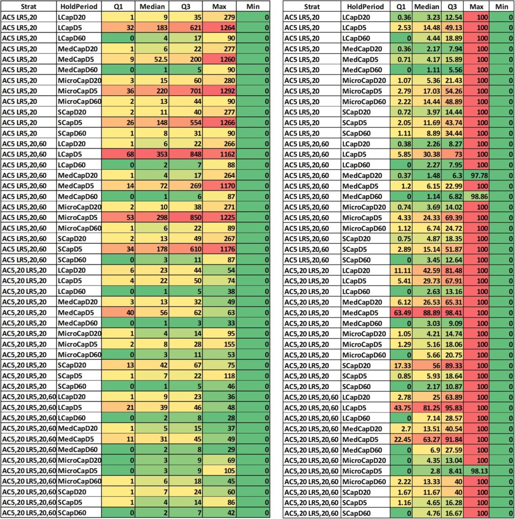
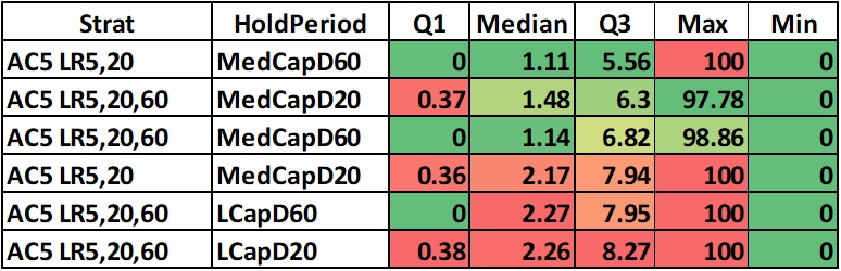
2. Draw down statistics: These are calculated as the number of trades within each returns path that had a value < 10000 (the starting capital of each returns path) – table below on left.
But since each returns path had different number of trades (depending on the signal criteria), it’s a good idea to normalize the drawdowns by the total number of trades – table below on right.

For example, in Large cap universe, with a signal of AC5 & LR5,20 and a holding period of 20 days, the median number of trades with drawdown was 9, and as a percentage of total trades was 3.23%.

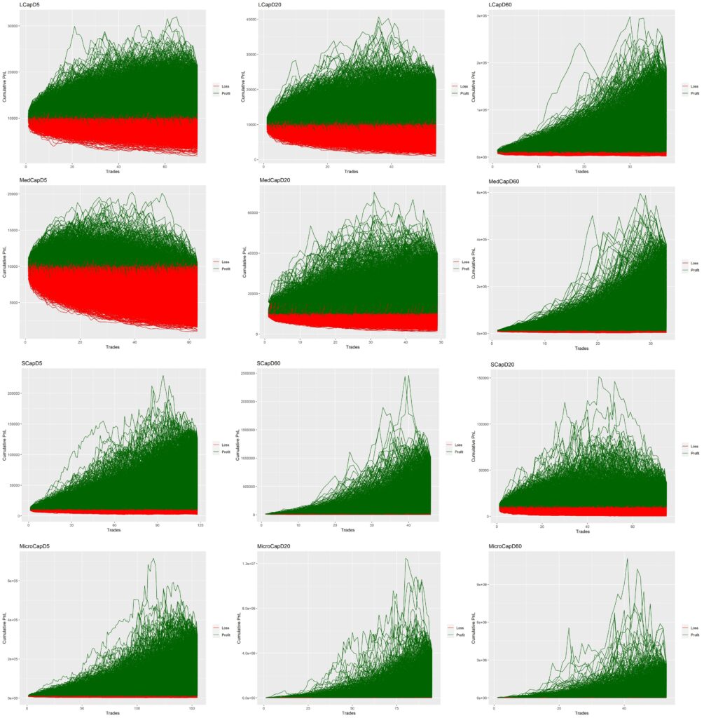
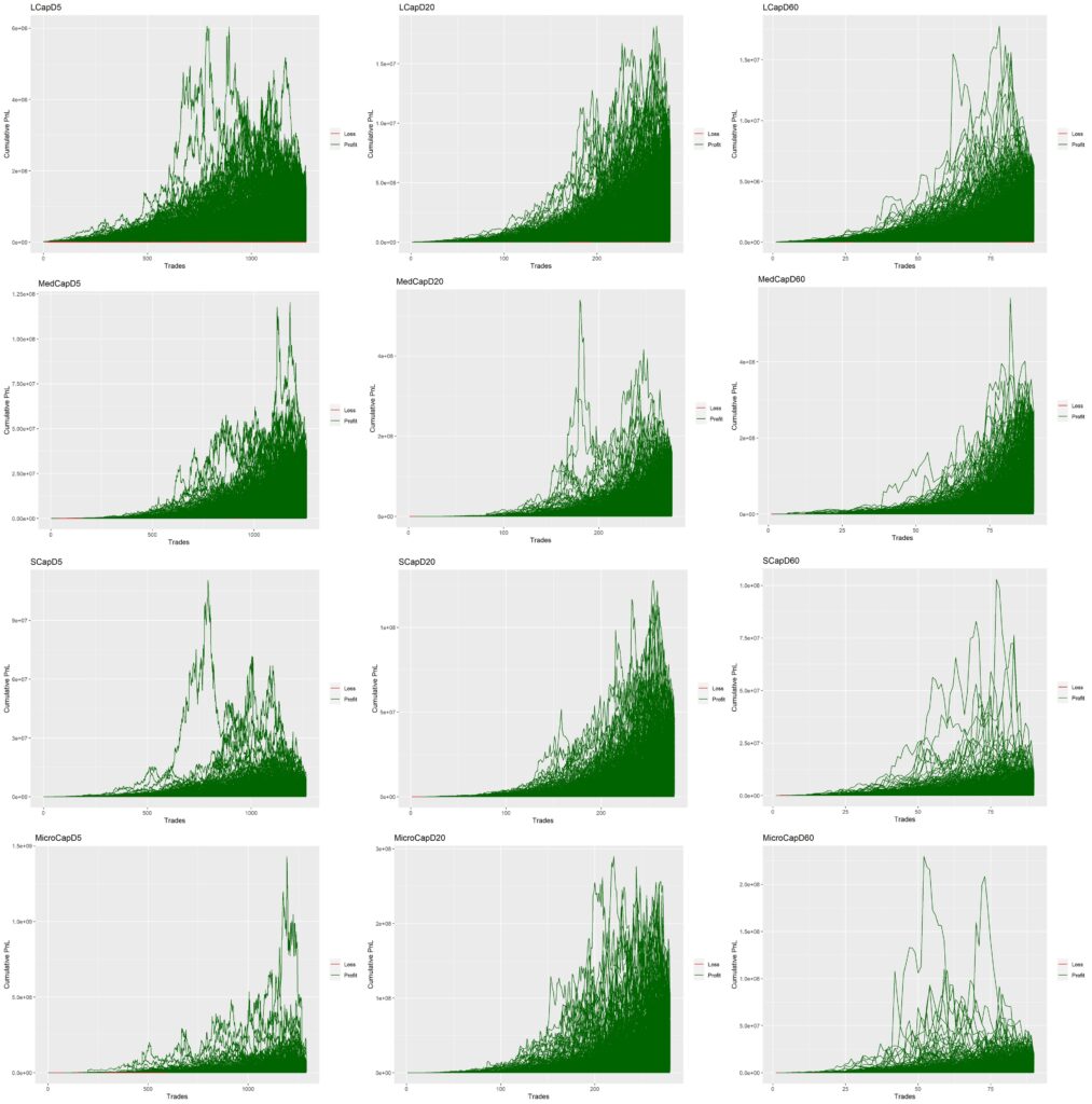
Finally, below you’ll find the returns paths of all the return streams computed within each strat/marketcap universe/holding period.

LR positive and significant for all windows (5/20/60D) and AC positive and significant for 5/20D windows

LR positive and significant for all windows (5/20/60D) and AC positive 5D window

LR positive and significant for 5/20D windows and AC positive and significant for 5/20D windows

LR positive and significant for 5/20D windows and AC positive for 5D window

DISCUSSION

From the first table (Final Return Statistics), we can quickly chuck out the strats which have a final 1st quartile return < Rs. 1,72,562 (the returns of 10k plunked into Nifty at the beginning of the backtest period). We are not using the median return against the benchmark, because we can afford to be selective, since we have so many strats to choose from. And using the first quartile gives us the strats in which 75% (approx) of the paths give us returns more than Nifty.
That leaves us with the following strats/marketcap universes/holding periods.

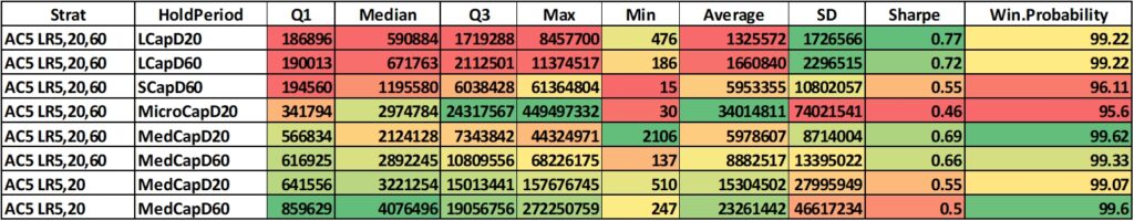
Immediately we notice that all the AC5,20 strats and holding periods of 5 days have been removed.
AC5,20 strats have a tendency to give the buy signal less often, and hence number of trades are less, hence final returns are less.
5 days holding period is also far too short for a stock to exhibit good returns.
Next we can narrow down the search using Sharpe ratios. This is a bit subjective, but I would cut out the strats which have a Sharpe < 0.6.

That leaves us with Stock universes of LCap and MedCap, bought via signal from AC5 & LR5,20,60 and held for 20 and 60 days.

Coincidentally, these four strats are among the lowest 3rd quartile drawdown percentages (table below). This makes us more sure of the choice of the strats.

These four strats would be the basis of the stock trend screener which is in the works following this.
I know that this article is a bit too long, but to do justice to a prolonged process, the length is necessary. I hope you found this useful. Please share the article with like minded friends and show some love. A lot of effort was put into this writeup.

Please let me know any criticisms or clarifications, on twitter or in the comments below. Until next time. Cheers.