INTRODUCTION
Since the relatively successful results of the stock trend screener (HERE), I have been obsessed with poking holes into it. I mean, something too good to be true, usually is. One of the criticisms I could think of (and has been pointed out by other astute observers on twitter), has been the fact the I start the backtest on one specific date (the first day of the data I have), and hold the randomly selected stock for a fixed period (5/20/60 days). That sort of brings in a calendar effect (the days during the hold period are completely missed out).
This is a major hang-up. We are literally missing the variation in returns that can happen if you selected the start of the backtest on some other day. This phenomenon is called “Rebalance Timing Luck”. In this post I try to observe whether this phenomenon exists with the AC5 LR5/20/60+ strategy of stock selection.
METHODOLOGY
The method of criteria generation, stock selection, hold period and random path generation is exactly the same as detailed HERE.
Except, I generate the random paths by starting the backtest on the missing days too (For example, for 5 day holding period strat, I generate separate paths for day 1,2,3,4,5 from the first day of backtest – “02-01-2002”).
For each missing day 50 random paths are generated via random stock selection, and each of those paths is scrambled via bootstrapping to generate 10 paths per original path, to randomize regime related effects on compounded equity curves.
Thus for 5-day holding strat, I end up with 500 paths for each starting day. Hence 5*500=2500 paths for 5-day holding strat.
Similarly, 20-day holding produces 50*20*10=10000 paths.
And, 60-day holding period produces 50*60*10=30000 paths.
Every step of this exercise is repeated for Large cap, Mid cap and Small cap universes.
After computation of the paths, we end up with final compounded returns distribution of 255 unique starting days and holding periods for all three marketcap universes. Visualizing individual paths with this many unique combinations is a fallacious time waste of an exercise (observing 255 separate masses of green and red lines isn’t really useful). So I decided to only focus on the final returns and their distribution.
RESULTS & DISCUSSION
The hypothesis we wish to disprove is that returns from all the separate backtest initiation days are going to be similar.
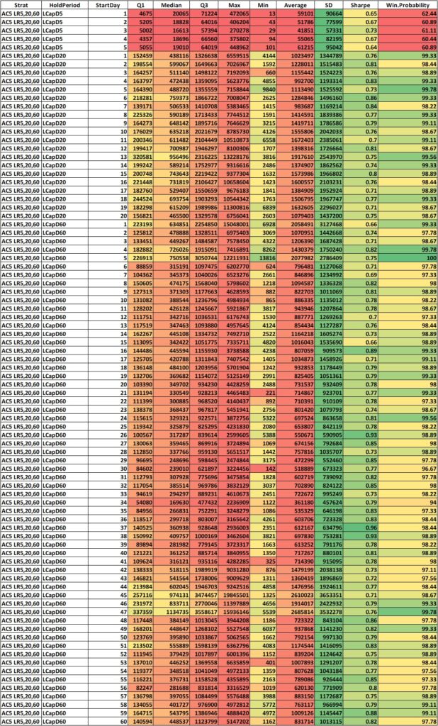
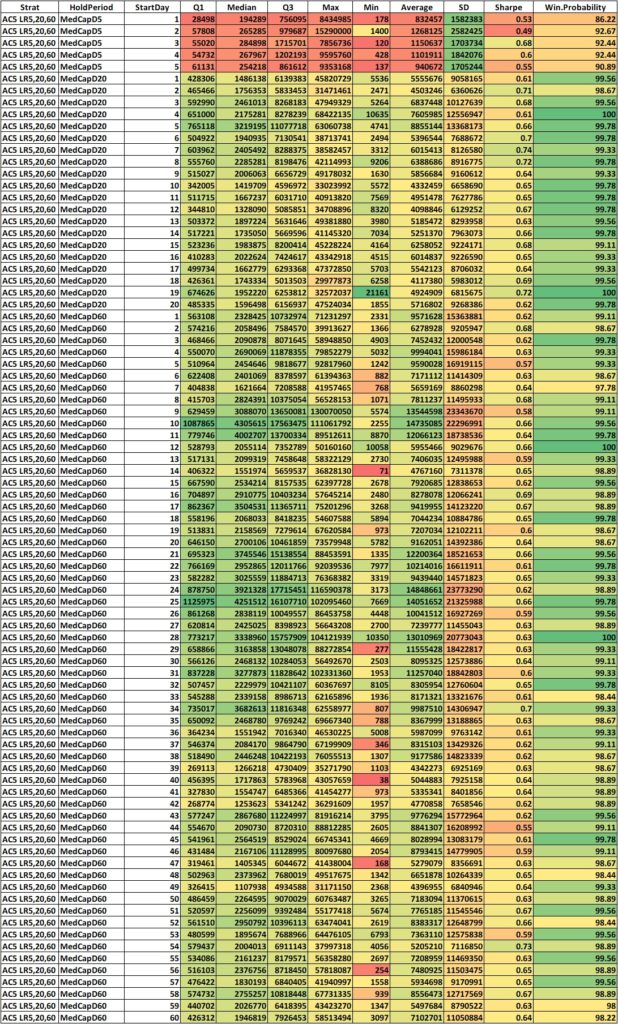
First let us look at the descriptive statistics of the same. Below you’ll find long tables of descriptive statistics of cumulative compounded returns of each the holding periods with different starting days, for separate marketcap universes.
LARGE CAP
MID CAP
SMALL CAP
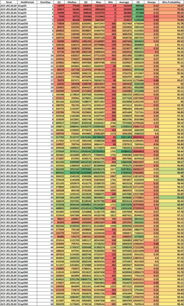
Wow! That’s a lot of numbers. Even visualizing the descriptive statistics is a massive task. Even after giving them a color gradient, it is difficult to see if the returns are different within each holding period, between the starting days.
Let’s look at it from a different perspective. Let’s try and qualitatively compare the probability density of returns for each of the holding periods. If the term “probability density” seem confusing to you, please refer to THIS ARTICLE.
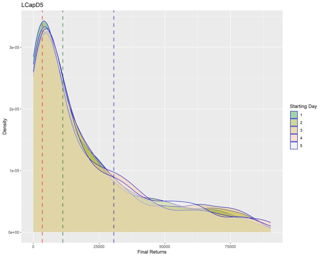
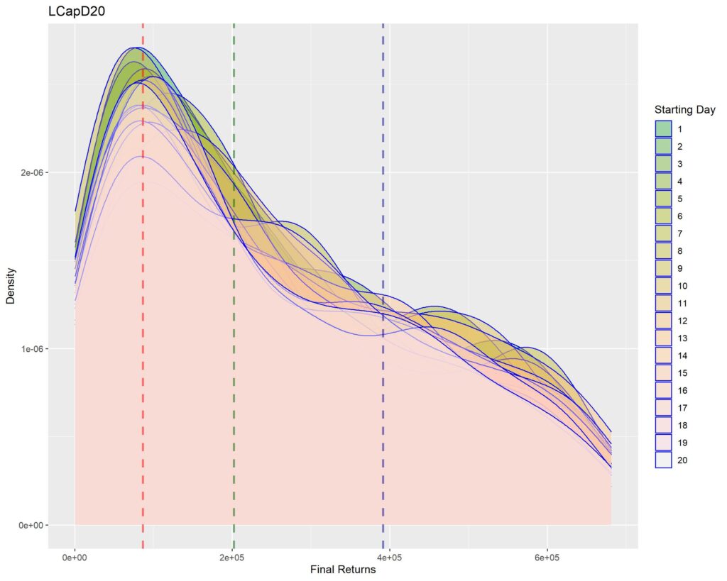
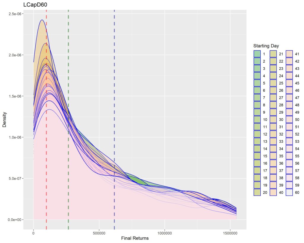
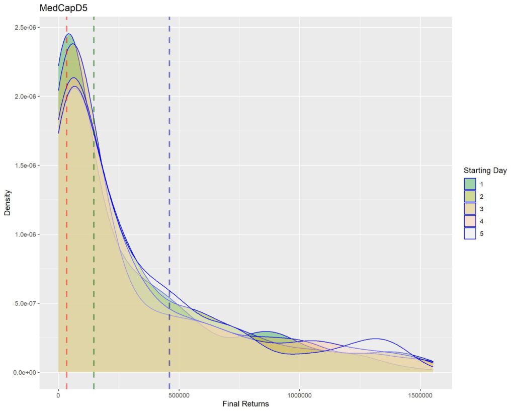
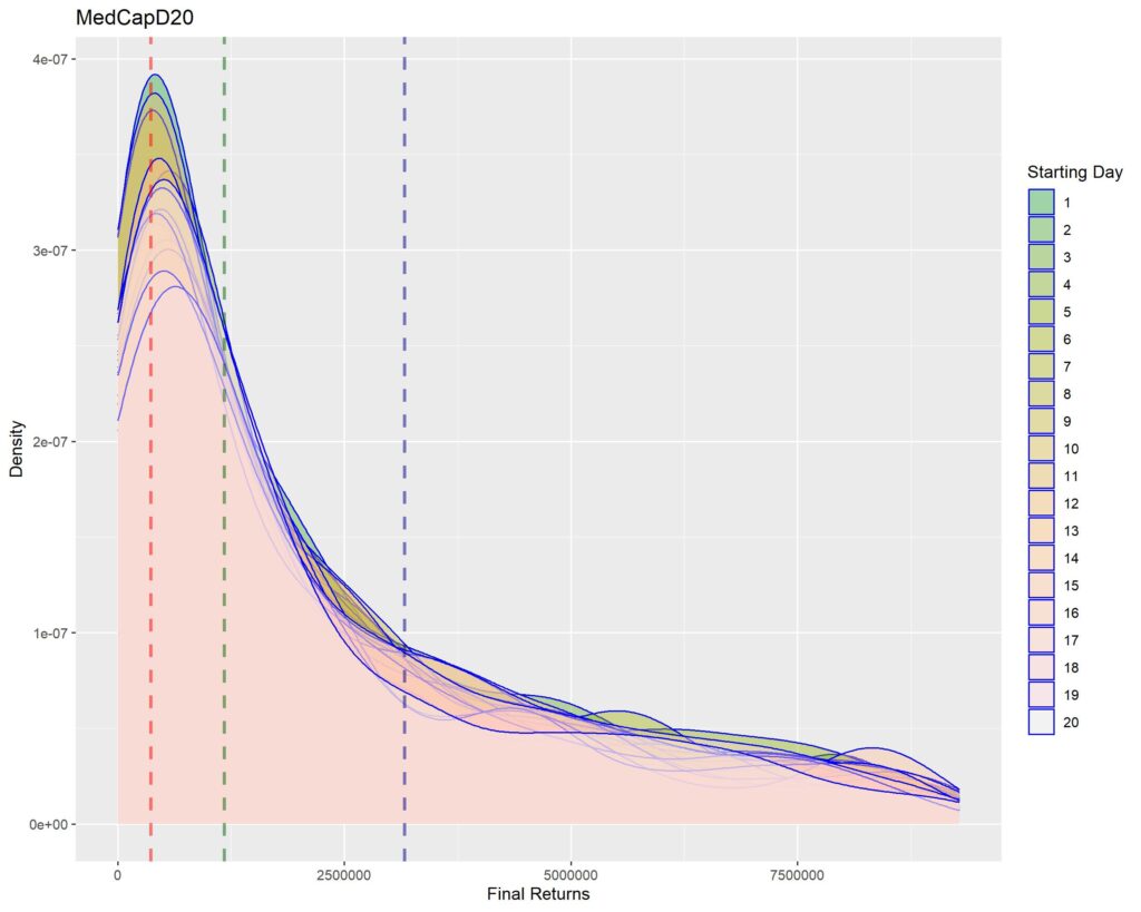
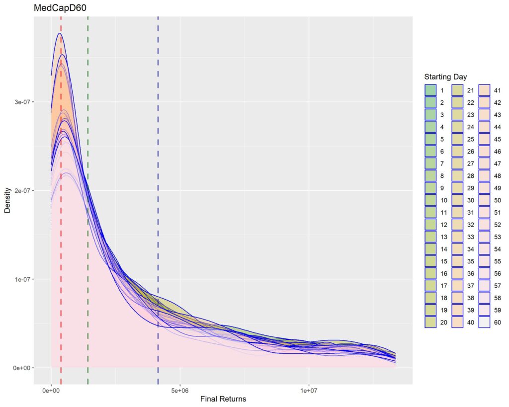
Below you’ll find graphs for the same. The vertical dotted lines are first quartile (red), median (green) and third quartile (blue) of returns within that strat cohort.
LARGE CAP
MID CAP
SMALL CAP
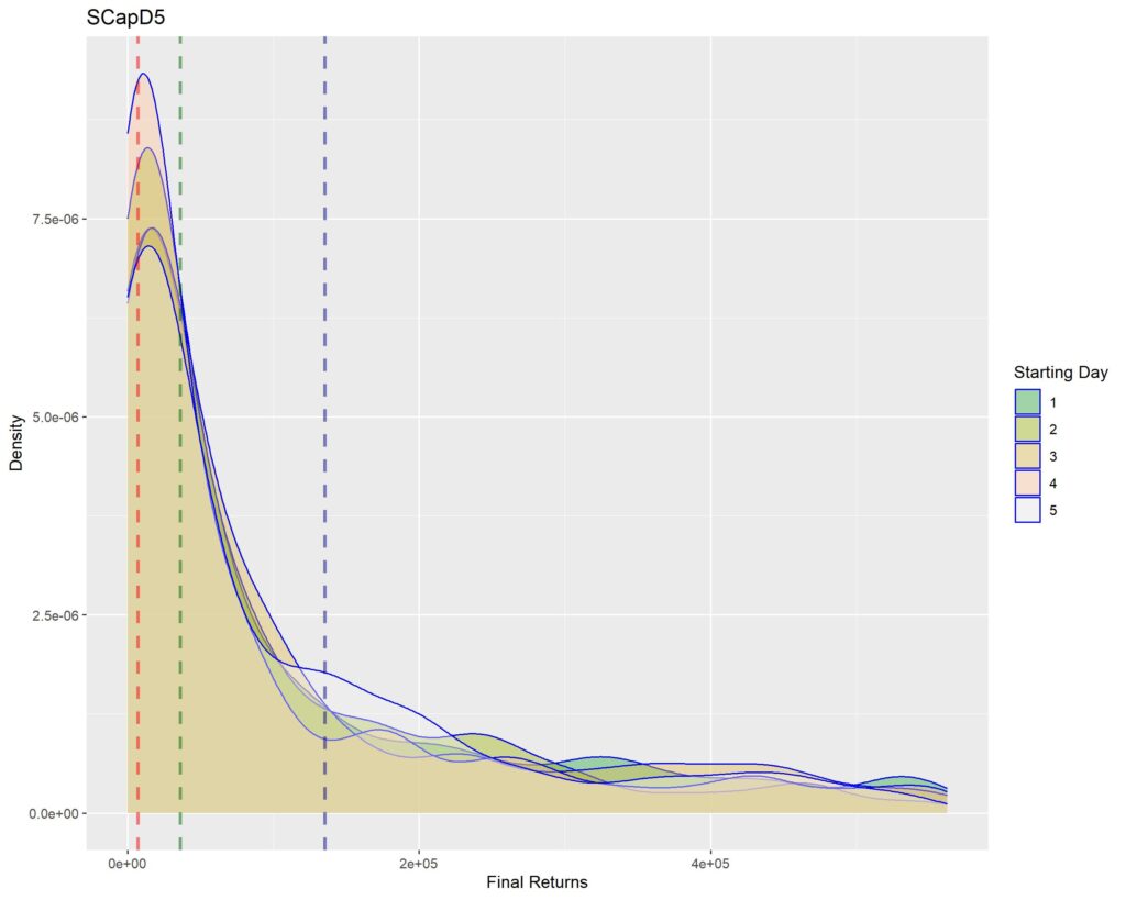
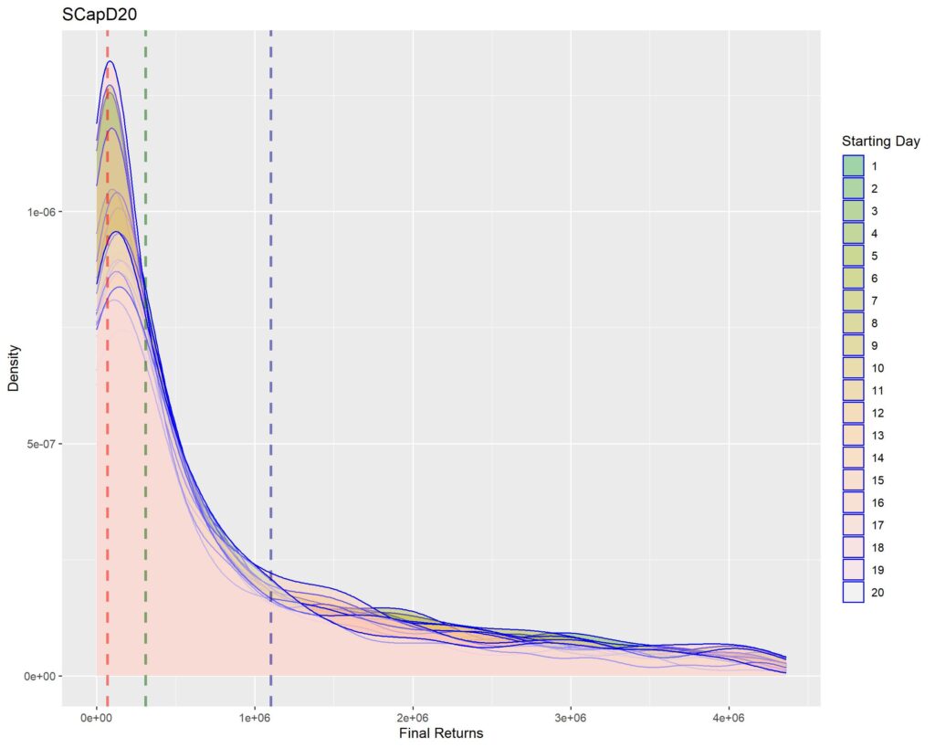
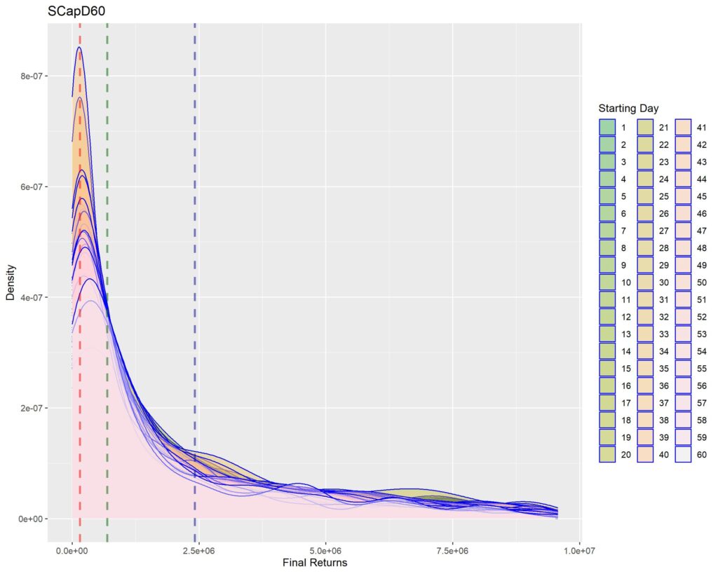
Interpretation of density graphs:
1. A sharper peak with rapid roll-off means that the probability of getting a higher return rapidly reduces (or simply, most of the times you’ll have returns similar to the peak – probabilistically lesser chances of higher returns for sharper peaks). Thus broad density distributions such as the ones for LCap20 are the strats where you’ll fare better. SCap ones are too narrow to be of any use to us.
2. In all the graphs, density peak mostly coincides with the first quartile line (dotted red). This shows that if we select a strat based on median returns, you’ll be doomed to failure. The median is around the place where the probability of higher return rapidly tails off. This is one of the reasons of why we used Q1 as the benchmark in the Path Analysis Article, for selection of useful strats.
3. Density graphs for separate starting days should be closer together if return distributions are to remain similar (closer blue outlines is better). Returns are not as much dependent on Rebalancing Timings if the density graphs are more cohesive. However, we see that the cohesiveness is more in D5 strats than in longer holding periods. This is expected, as more variability will be introduced if more days are tested. Overall, we can’t tell much about this timing dependence just by looking at the graphs.
Thus, we need to dig a little deeper into statistics for getting better answers.
We will try two ways of looking at this,
1. Group tests: We assume that final returns of each of the starting days are independent from other starting days. And we try to see if the returns are statistically different among them. Since we cannot assume a normal distribution for the returns, we go for a rank based non parametric test called “kruskall wallis” test. If the p-value generated by this test is <0.001, we can say that there is less than 0.1% chance that the returns are similar for all the starting days.
2. Variance attribution: In this we try to observe how much of the variance of final returns is explained by the starting days. This will be done by constructing a linear regression model (can also be done using ANOVA, but I’m just lazy and syntax for linear regression is easier), with final returns as the predicted variable and starting days as the predictor variable. Starting days have been assumed to be independent categories within themselves for this analysis and taken as nominal for this analysis. Then r-squared of the model is calculated to get the variance attribution. The number should be read as percentage of variance of final returns being explained by the change in starting days.
The table below shows the results.
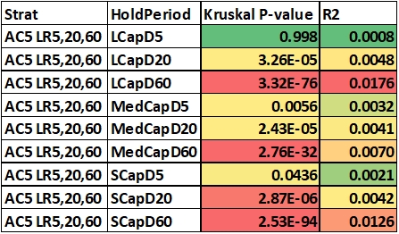
Immediately we see confirmation of what we observed in the density graphs. Returns from D5 holding periods are almost similar (P>0.001). While r-squared (R2) is also lower for the same.
While 20/60 day holding periods have significant differences between the starting days (P<<0.001), for all marketcap universes.
But if we look at the variance attribution (R2), maximum explained variance is in LCapD60 (1.76%) and most all are below 1%.
Thus although the difference is statistically significant, it may not be that bad for us if we stick to the strats where even Q1 final returns are above Nifty buy and hold.
CONCLUSION
I concede that this is a stats heavy article. But the approach may be found useful as refinement procedure for strats with positive expectancy and higher than benchmark returns.
In conclusion, though the rebalance timing can definitely affect the eventual returns, probability is on our side if we use the strats with Q1 returns above Nifty. Those are the same strats defined in the Path Analysis article.
If you found this useful, please share with your comrades.
If you found it confusing, please fell free to ask questions below in the comments, or by contacting me on twitter – https://twitter.com/Dhritiman_Ch.
Until next time, Cheers.