Statistical Testing for Trading Strategies

This blog piece is based on questions asked to me a while back by Gaurav Rungta (@grt_0101) on twitter. The question was regarding t-test and its utility in context of backtests. While this can be treated as a super expansive topic, I’ll try to approach this from a very basic perspective so that maximum people are benefited.

Any hypothesis test that we conduct always starts with a nihilistic point of view. That the stuff we are testing for doesn’t exist in real life. That nihilistic view is termed “null hypothesis”. What we need to test for is the optimistic view point called “alternative hypothesis”.  

For a simple example consider the the following sample of returns from a trading strategy: [-0.532, 0.698,  0.168,  0.268,  1.118,  1.838,  2.928,  0.508,  2.888,  0.118,]. Just by looking at it, we cannot tell whether the strategy overall has a positive expectancy. Our question here can be simply stated as “Does my strategy have a return > 0% return?”.  That’s a good question, but a better question would be in two parts:

1. “Does my strategy have a return > 0% return?”
2. “How sure am I of these returns and will be returns be similar if I used this strategy over longer periods?”

The first part of the question can be easily answered by reducing the data series into few understandable values. Those understandable values can be termed “measures of central tendency” and “measures of dispersion”. The former includes Means and Medians. The latter includes Variance and Standard Deviation (SD). We’ll stick to the more commonly used ones – Mean and SD. The above data series has a Mean of exactly 1 and an SD of 1.19. That tells you that based on your modeling (reducing data to understandable parameters), the returns vary between -1.38 and 3.38, 95% of the times in your data. These numbers are calculated from Mean- 2*SD and Mean+ 2*SD and based on assumptions that we need not get into right now.

You could happily accept these results as the absolute truth, but frankly that would be idiotic. A better method would be conducting this experiment 1000 times in the similar fashion (either collect historical data of 10 consecutive returns, randomly sampled; or use the strategy prospectively and collect live data), and see whether these returns are repeated in a similar manner or not.

What you’ll notice is that mean returns will be variable and chaotic. Doing this exercise will show you that the Mean return you originally had, is part of a larger universe of Mean returns from other points in history/future. And which mean return you get when you trade the strategy live is completely random. Hence comes importance of the second question – How sure are you of your Mean return?

For that you need to understand the two opposing forces acting on your conviction:

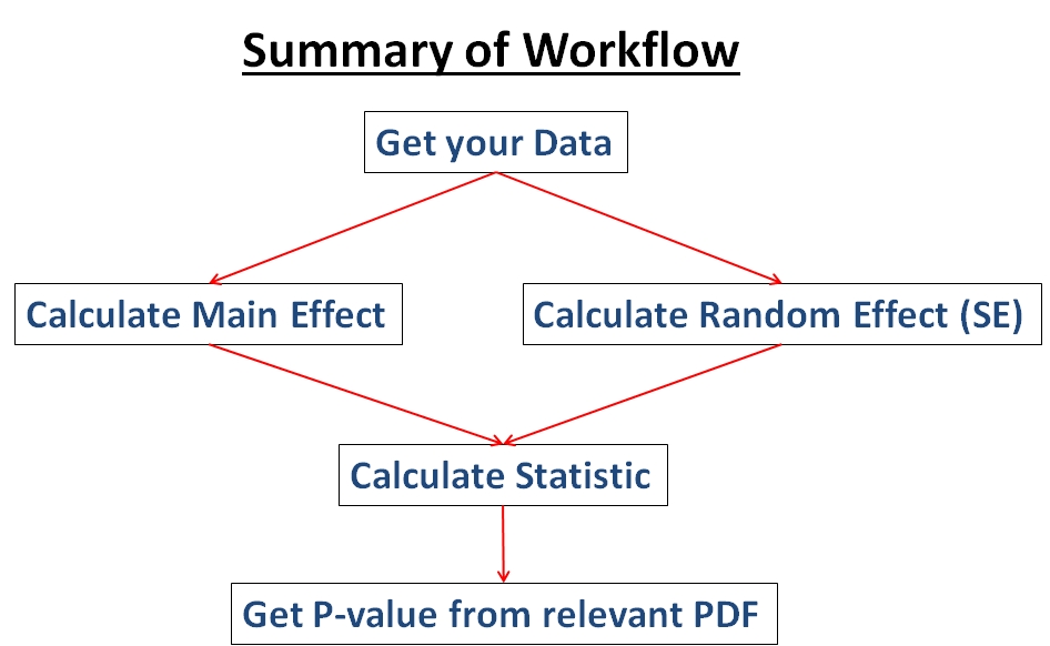
1. The true alpha of your strategy (hereby termed “Main Effect”)
2. The uncertainty of your strategy delivering promised Main effect repeatedly (hereby termed “Random Effect”)

If you wish to model this conviction to a single number, simply create a ratio – Main Effect/Random Effect. Higher this number, more is your conviction. In traditional statistics tests, this ratio is called a “Statistic”. Like Z-statistic (for normal distribution), T-statistic (for T distribution – beefed up normal dist), F-statistic (for F distribution) etc. Probability distributions are a larger rabbit hole that you shouldn’t dive into right now. But for those interested, just use wiki and follow the links (that’s what I’d done) – https://en.wikipedia.org/wiki/Probability_distribution.

The Random Effect in hypothesis tests is encapsulated in the term “Standard Error” (SE). There are various ways of calculating this standard error for different hypothesis tests (again not discussing for brevity). For our purpose, we’ll want to see if the Mean of 1 with SD of 1.19 gives us conviction that our returns will be different from 0 in the future. For this we do a standard Z-test (though we shouldn’t coz the sample is too small to assume a normal dist). SE of z test is calculated as: SD/sqrt(N).
From this we calculate the aforementioned ratio – Z statistic: (Main Effect – Null Effect Mean)/SE. So for our purposes, it comes out to (1-0)/(1.19/sqrt(N)) = 2.66. This is our scale-less measure of conviction. Now how does this number help us?

This number can be used as a metric to see the probability of our effect being different from null effect (this is where probability distribution comes into picture, but we will ignore it). For traditional tests, there are ready-made functions which compute this probability (in Excel it is Z.TEST). From this you get a metric called “P-value”. This number gives the “percentage of times your returns will be same as 0, if you repeated the experiment/strategy infinite times”. The cut-off of P you want to use is up to you, but a thumb rule is to accept the strategy if your P is less than 5% or 0.05. For our strategy it came 0.008, so I would say that this strategy is significantly different from not doing anything, hence viable. What we have accomplished until now is called a single-sample test (tested against a fixed NULL).

But getting a significant P-value from a small sample isn’t the holy grail. What you need for further conviction is to increase your sample size to increase variability in your data, incorporate outliers and then see if it still works. Beyond that is to compare the returns against Nifty/other standard strategy, for which you’ll need to do independent samples test (tested against another population – sort of variable NULL). For this the alternate hypothesis becomes – “is the mean of difference of returns, different from 0”.
For both these tests, we are assuming that each unit of return (each daily return) is an independent entity – which might or might not be true. But that’s whole another rabbit hole.

Hope this was useful. Cheers.